Classic Hexbeam - In depth
On this page we will explore some of the technical details behind the Classic Hexbeam. In particular we will look at which of the antenna dimensions are critical to particular performance parameters. Here's the "Executive Summary":
- Reflector dimensions determine the tuning of the antenna
- Driver dimensions largely determine the feedpoint impedance of the antenna
- End spacing affects tuning and the peak F/B performance
- Wire gauge affects tuning and SWR, and needs wire dimensions to be modified
1. How does it work?
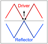
The principles behind Hexbeam operation are no different than those of any 2-element "parasitic" beam. One element - approximately half a wavelength long - is "driven" by the transmitter; the other - also about a half-wavelength long - is placed close to the driven element. As a result of its proximity, currents are induced in this second element which result in power being re-radiated from it; because it is not driven directly this element is called "parasitic".
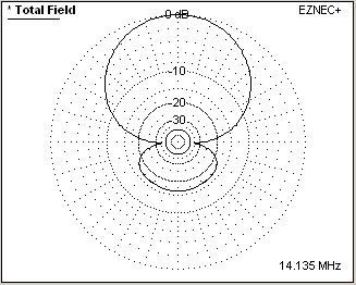
The relative magnitude and phase of the currents in the parasitic element result in the "re-radiated" power reinforcing the power from the Driver in some directions, whilst cancelling it in others - hence the antenna becomes "directional". In a Classic Hexbeam the Front-to-Back ratio peaks at the self-resonant frequency of the Reflector. The Azimuth plot on the right shows the directionality that is typical of the antenna.
The challenge to the antenna designer is to control the "mutual coupling" between the elements in such a way that the relative magnitude and phase of their respective currents optimises the antenna's performance. In the case of the Hexbeam this "mutual coupling" is controlled partly by the general spacing between the elements, and, critically, by the gap between the tips of the Driver and Reflector.
If the designer had total control of the relative magnitude and phase at all frequencies, excellent Hexbeam performance would be possible over a wide bandwidth - gains in excess of 6.8dBi (4.7dB more than a dipole) and F/B ratios over 40dB. But of course in the "real world" such control is not possible, so before getting too carried away we need to manage our expectations!
2. Yagi performance
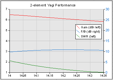
The chart on the right shows the modelled performance of a full-size 2-element 20m monoband yagi in Free Space; it makes a useful reference for judging the performance of the Classic hexbeam.
This Yagi has a 386" Driver, a 418" Reflector, and a 133" boom length (0.16 wavelengths) - a typical compromise between Gain, Front-to-Back ratio (F/B) and a reasonable match to 50 Ohms. The antenna has an 18.3ft turn radius and is assumed to be constructed from 3/8 inch diameter aluminium
We see that the full size Yagi is a relatively broadband antenna. The Gain falls by only 0.7dB across the 20m band and never falls below 5.8dBi. The F/B varies by only 1dB across the band, peaking at 11dB. On the other hand, the SWR varies significantly from 2.1 at the lower band edge to 1.0 at the top of the band.
So, what can we reasonably expect from a Classic Hexbeam just over half the Yagi's size?
3. Classic Hexbeam performance
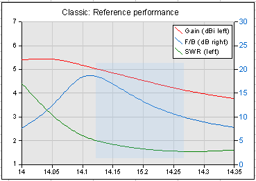
This chart shows the performance of a typical 20m monoband Classic Hexbeam. Each Driver leg is 219" long and each Reflector leg is 222". The spacing between the Driver and Reflector tips totals 11" and it is constructed from #16 gauge bare copper wire; it has a turn radius of 9.4ft. The dimensions were chosen to provide a good compromise between Gain, F/B and SWR. This antenna will be used as a benchmark as we explore the effect that various dimensions have on Classic Hexbeam performance.
The first thing we see is that the Hexbeam has less Forward Gain than the Yagi, and the Gain falls by 1.7dB across the band - a result that is typical of end-coupled wire beams. At the top of the band, the Gain is 2dB (1/3 of an S point) below the Yagi, but we might judge this is a reasonable price to pay for the reduction in size.
The Hexbeam beats the Yagi for peak F/B at 18dB; however the F/B falls to 7.5dB at the band edges, and so maintains its advantage over only 60% of the band.
The SWR falls quickly as the frequency increases, but is still over 2:1 where the F/B is best. It is important to understand this characteristic of the Classic Hexbeam; constructors who tune their beams for minimum SWR are likely to be disappointed by the directivity of the antenna. This poor SWR characteristics is caused by an abrupt drop in the resistive component of the feedpoint impedance at frequencies below the peak F/B.
If we define "useful performance" to mean Gain>4dBi, F/B>10dB and SWR<2, we find that the Classic Hexbeam has a useful bandwidth of just 150KHz on 20m as shown by the shaded area on the chart. This makes it imperative that we tune the antenna to optimise the performance at our preferred operating frequencies.
Despite the narrow bandwidth, the Classic hexbeam compares very well with commercial HF mini-beams. For example, according to figures published by Cushcraft, the 20m Gain of the MA5B is 3.6dBi and its 2:1 SWR bandwidth is 90 KHz.
Now let's explore which of the Classic Hexbeam's dimensions are critical, and how they affect its performance.
4. Reflector

The length of the Reflector on a Classic hexbeam has little effect on Gain and peak F/B, but it has a pronounced effect on the tuning of the beam (i.e. the frequencies where it delivers maximum Gain and best F/B ratio). It also has some effect on the SWR, as a result of the Driver / Reflector ratio changing, but it is small compared to the effect on tuning.
If we change the length of each Reflector leg on our reference antenna from 220" to 224" in 1" steps and plot the F/B ratio at each step, we get the results shown on the right. We see that for each 1" increase in Reflector length the frequency of peak F/B drops by about 68 KHz. And because 1" represents 0.5% of the leg length, whilst 68KHz is 0.5% of the centre frequency, we conclude that Classic hexbeam tuning is linearly dependent on Reflector length at a rate of 68KHz per inch.
By extrapolation we can calculate equivalent numbers for the other HF bands which are useful to remember when you are tuning your Classic Hexbeam:
- 20m - 68KHz/inch
- 17m - 108KHz/inch
- 15m - 146KHz/inch
- 12m - 202KHz/inch
- 10m - 256KHz/inch
Getting the Reflector length right is essential if a Classic HexBeam is to perform well. It is the most critical of all the antenna's dimensions.
5. Driver


The length of each Driver leg on our reference antenna was changed from 217" to 221" in 1" steps; the Gain, F/B and SWR were noted at each step. There was a negligible effect on the Gain, the F/B performance or the antenna tuning, but there was a significant effect on the SWR as shown on the right. Shortening the Driver has improved the SWR at higher frequencies, but worsened it at lower frequencies where best Gain and F/B are delivered. Unravelling what has caused the change in SWR is important because it provides an understanding of how the Driver length affects the feedpoint impedance of the beam, which in turn allows us to tailor the Driver to meet particular matching requirements.
The second chart shows how the Gain, F/B and Feedpoint Impedance of our reference antenna change as we alter Driver length over an extended range of 213" to 223"; the parameters are all measured at the frequency of peak F/B. We note that:
- directivity and tuning are substantially independant of the Driver length;
- the resistive component of the feedpoint impedance is steady at around 24 Ohms;
- the reactance increases linearly - each 1" adding about 7 Ohms.
In passing, notice that the beam still performs well when the Driver is longer than the Reflector (222") ! This may seem rather strange if you are used to dealing with conventional Yagis where the correct Reflector / Driver ratio (R/D) is key to establishing the proper phase relationship between their currents to produce directivity. This is not the case with the HexBeam (and other beams such as the VK2ABQ) where the end coupling is the critical factor.
Typically, values of R/D between 1.015 and 1.02 (equivalent to 219" and 218") are used in Classic Hexbeam designs because they result in reasonable SWR figures. But the chart shows that more extreme ratios can be used, without detriment to antenna performance, where necessary to meet certain matching requirements. A very useful ratio is 1.04 (equivalent to 214" on the chart) which results in a feedpoint impedance of about 25 - j25 Ohms - a value which can be translated to an SWR near unity using a "Beta Match".
6. End Spacing

The total End Spacing on the Reference model was changed from 3" to 19" in 4" steps; at each stage the Forward Gain, SWR and F/B performance were noted across the band. The F/B figures are shown on the right. We can see that changing the End Spacing had some effect on antenna tuning - presumably because the closer spacings detune the Reflector low in frequency. Closer spacings also made a small improvement to the SWR. However, the major impact was on the peak value of F/B.
We might be tempted to opt for a large End Spacing in pursuit of the highest peak F/B performance. However, the F/B performance is little better at the band edges with the larger spacings, and detailed analysis of the azimuth patterns shows that the high F/B numbers can be somewhat illusory. In some instances they result from deep, narrow, "notches" in a cardioid pattern which may not be particularly useful in day to day operation. So if we opt for a more "modest" spacing, like 11", we shall lose little practical F/B performance and will benefit from a slightly lower SWR.
7. Wire gauge

Wire gauge affects all Classic hexbeam performance parameters other than SWR to an extent: thicker wire improves forward Gain because it reduces copper losses; it tunes the antenna higher in frequency; but it reduces peak F/B because it increases the Driver / Reflector end coupling.
The chart on the right shows the effect on F/B of stepping the wire gauge from #12 to #20. We can see the reduction in peak F/B from 21dB to 17.5dB that this caused, and also the 120 KHz shift in tuning.
There is probably no overriding reason to use one wire gauge rather than another. Choosing a thinner gauge such as #16 loses a little forward Gain, but it improves the peak F/B and results in a lighter antenna. If any other gauge is used, the Driver and Reflector dimensions must be scaled as explained in Wire size and type.
8. Matching the Classic Hexbeam
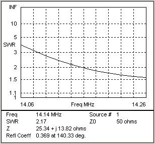
As a reminder, the chart on the right shows the sort of SWR characteristic we can expect from a Classic Hexbeam across the 200KHz band where it shows best directivity. The SWR falls from 4:1 to 1.5:1 across this band. At the lower frequency limit the beam's impedance is [13 + j3] Ohms, rising to [38 + j16] Ohms at the upper frequency limit. Mid-band the impedance is [25 + j14] - an SWR of 2.2:1
It may be that, if your rig has an automatic ATU or that you are prepared to operate through an external ATU, you can cope with the SWR without needing to introduce any matching at the antenna. If not, there are a couple (at least) of simple matching techniques that can be used with a monoband Classic Hexbeam.
a) Series matching section ( 25 Ohm line )
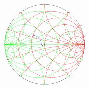
On the Smith Chart to the right we have plotted at Point 1 the typical impedance presented by a Classic Hexbeam mid-band [25 + j14]. The chart shows the effect of introducing a series section of transmission line having a Characteristic Impedance (Zo) of 25 Ohms and an electrical length of 0.1 Lambda. The impedance has been transformed to [43 + j0] at Point 2 - a reduction in SWR from 2.2:1 to 1.2:1
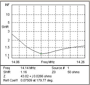
If we now introduce this series transmission line section into our model we can see its effect on SWR across the frequency range of interest in the second chart. The SWR has been improved to below 2:1 in all but the bottom 20KHz of the range. The SWR at 14.060 MHz could probably be reduced to below 2:1, at the cost of a small increase at 14.260 MHz, by small adjustments to the length of the series matching section.
25 Ohm line is not something that is readily available commercially, but can be fabricated easily by "parallel connecting" two identical lengths of 50 Ohm line. Connect the inners of the coax together, and the braids together, at either end of the run. Make sure the two lengths of line have the same velocity factor!
To summarise the technique:
Add two parallelled lengths of 50 Ohm coax
between the beam and your main 50 Ohm feedline; make the parallelled lines one
tenth of a wavelength long, remembering to take account of the velocity factor.
For example, at 14.140 MHz the length would be about 4.6ft.
b) Beta matching using a shortened Driver
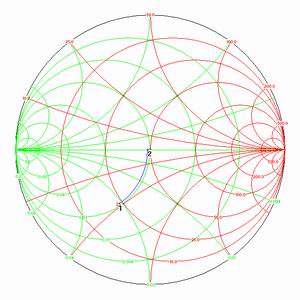
Earlier on this page we learned that the Driver of the Hexbeam could be shortened or lengthened considerably without compromising the performance of the antenna. Shortening the Driver caused an increasingly capacitive component at the feedpoint; we noted that for a Reflector / Driver ratio of 1.04 the impedance was about [25 - j25] Ohms which makes it a prime candidate for Beta matching. This impedance is plotted as Point 1 on the Smith Chart to the right.
Adding parallel inductance is equivalent to moving around a circle of "constant conductance" on the Smith Chart, so we are easily able to transform Point 1 into Point 2 - a new impedance of [48 + j0]Ohms and an SWR close to unity - by placing a coil across the feedpoint of the antenna. This inductor needs to have a reactance of 50 Ohms - about 0.57uH at 14MHz.
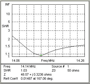
If we now model the shortened Driver with the parallel inductor we can see the effect on SWR across the frequency range of interest in the second chart. The SWR has been improved to below 2:1 in all but the bottom 10KHz of the range. Small adjustments to the inductor would likely improve the SWR at 14.140 MHz to below 2:1 at the cost of some small increase to the SWR at 14.260 MHz.
To summarise the technique:
Make the Driver 4% shorter than the Reflector
and add an inductor with a reactance of 50 Ohms across the antenna feedpoint
(e.g. 0.57uH for 20m)
9. Baluns
Many HexBeam users wonder whether or not to include a balun in their feedline. I recommend the use of a 1:1 choke balun: when I added one to my beam I noticed that measured SWRs were more "repeatable" and less dependent on the route taken by the feedline. I use a ferrite choke balun, but a "coiled coax" choke would likely be as effective. If you build one don't overdo the number of turns: for 20m through 10m, 6 turns of RG213 on a 4" diameter former is plenty.